This project was completed as part of Google Summer of Code 2019 under the mentorship of RedHen Lab. I’d like to thank Prof Dr TM Thasleema, Central University Kerala and Karan Singla, PhD graduate student at USC Viterbi school of Engineering, mentors of this project for their extended and comprehensive support without which this project wouldn’t have been completed. Also absolutely indebted to Prof Mark Turner, Case Western Reserve University, and Prof Francis Steen UCLA, for exceptional and quick support from the community side.

The scope of this project is to build a generic high accuracy Speech Recognition engine using Deep Learning to understand English news and specifically Indian English news.

Datasets

As Deep learning based Speech Recognition engines require high amount of data to converge, this model was trained on a large volume of data, which includes :

• NPTEL : Indian video lecture series, 1000 hours of which was processed and transcribed and was used for training.

• Fisher : Noisy conversational Speech dataset of 1750 hours

• LibriSpeech : 1000 hours read audio book dataset.

• AMI : close mic 100 hour meeting dataset.

• Switchboard : 250 hours noisy conversational dataset.

• Tedlium : 500 hours of Ted Speaker dataset.

Languages & Frameworks

This project was completely developed in the Kaldi Toolkit, and was run, tested and deployed in a Linux Ubuntu variant OS. The languages used include :

• Shell

• C

• Perl

• Python

• Cpp

Timeline

• Week 1 : The first week was spent on setting up the workspace in Red Hen Gallina space. This was done in accordance with the Red Hen guidelines (here)[http://www.redhenlab.org/home/tutorials-and-educational-resources/using-singularity-to-create-portable-applications]. The Singularity image was setup, followed by installation of Kaldi then the datasets were downloaded and formatted according to its structure.

• Week 2 - 3 : Spent on pre-processing the English Datasets. Around approx 3000 hours of data was pre-processed and cleaned and made into a unified structure. Followed by feature extraction, initial HMM - GMM training.

• Week 4 - 5 : DNN training was completed in this stage. This was trained on a Google Cloud machine with 8 GPUs and has to re-iterate various stages for correction and accuracy improvements.

• Week 6 : Focused mainly on obtaining datasets for Hindi from LDC-IL at CIIL.

• Week 7 : Focused mainly on building the Hindi ASR project with pre recorded 200 utterances spoken by 6 different speakers.

• Week 8 : Completed the documentation and deployment of the project. Source code is available in Github . And the entire files has been uploaded to the the Red Hen Gallina Server. Available at : /mnt/rds/redhen/gallina/home/sxk1497/gsoc2019

Development

The development of the project was completed in multiple stages. The first step was to bring all datasets to a unified format which Kaldi understands. The first initial step was to create a unified pronunciation lexicon for all the words in the corpus using G2P tool, inclusive of the Fisher, Switchboard and NPTEL data.

if [ $stage -eq 1 ]; then
  # We prepare the basic dictionary in data/local/dict_combined.
  local/prepare_dict.sh $swbd $nptel
  (
   steps/dict/train_g2p_phonetisaurus.sh --stage 0 --silence-phones \
     "data/local/dict_combined/silence_phones.txt" data/local/dict_combined/lexicon.txt exp/g2p || touch exp/g2p/.error
  ) &
fi

Followed by which the next step was to create a unified structured dataset, or preparation of all datasets to a single format in which Kaldi work in. For this :

if [ $stage -eq 2 ]; then
  mkdir -p data/local
  # fisher
  local/fisher_data_prep.sh $fisher
  utils/fix_data_dir.sh data/fisher/train
  # swbd
  local/swbd1_data_prep.sh $swbd
  utils/fix_data_dir.sh data/swbd/train
  # librispeech
  local/librispeech_data_prep.sh $librispeech/LibriSpeech/train-clean-100 data/librispeech_100/train
  local/librispeech_data_prep.sh $librispeech/LibriSpeech/train-clean-360 data/librispeech_360/train
  local/librispeech_data_prep.sh $librispeech/LibriSpeech/train-other-500 data/librispeech_500/train
  local/librispeech_data_prep.sh $librispeech/LibriSpeech/test-clean data/librispeech/test
  # nptel
  local/tedlium_prepare_data.sh $nptel


  #AMI 
  local/ami_text_prep.sh data/local/ami/annotations/
  local/ami_ihm_data_prep.sh vault/ami/wav_db/

fi

Followed by this, normalization of the transcripts and Out of Vocabulary word removal from the dictionary were performed. And then the Language Model is prepared. This is done using the SRILM toolkit that comes alongside Kaldi :

if [ $stage -eq 6 ]; then
  mkdir -p data/local/lm
  cat data/{fisher,swbd}/train/text > data/local/lm/text
  local/train_lms.sh  # creates data/local/lm/3gram-mincount/lm_unpruned.gz
  utils/format_lm_sri.sh --srilm-opts "$srilm_opts" \
    ${lang_root}_nosp data/local/lm/3gram-mincount/lm_unpruned.gz \
    ${dict_root}_nosp/lexicon.txt ${lang_root}_nosp_fsh_sw1_tg
fi

Followed by which the feature extraction is performed on the entire datasets , the MFCC is generated in this stage :

if [ $stage -eq 7 ]; then
  mfccdir=mfcc
  corpora="ami_ihm fisher librispeech_100 librispeech_360 librispeech_500 swbd nptel"
  for c in $corpora; do
    (
     data=data/$c/train
     steps/make_mfcc.sh --mfcc-config conf/mfcc.conf \
       --cmd "$train_cmd" --nj 80 \
       $data exp/make_mfcc/$c/train || touch $data/.error
     steps/compute_cmvn_stats.sh \
       $data exp/make_mfcc/$c/train || touch $data/.error
    ) &
  done
  wait
  if [ -f $data/.error ]; then
     rm $data/.error || true
     echo "Fail to extract features." && exit 1;
  fi
fi

Followed by which the same is generated for test dataset as well. Then monophone training is completed. A monophone model is an acoustic model that does not include any contextual information about the preceding or following phone. It is used as a building block for the triphone models, which do make use of contextual information. Since this is a large dataset, in order to speed up, only first 10k short utterances from Switchboard was used for monophone training:

if [ $stage -eq 11 ]; then
 local/make_partitions.sh --multi $multi --stage 1 || exit 1;
 steps/train_mono.sh --boost-silence 1.25 --nj 80 --cmd "$train_cmd" \
   data/$multi/mono ${lang_root}_nosp exp/$multi/mono || exit 1;
fi

While monophone models simply represent the acoustic parameters of a single phoneme, we know that phonemes will vary considerably depending on their particular context. The triphone models represent a phoneme variant in the context of two other (left and right) phonemes. Hence triphone training is completed next stage by stage.

In first and second triphone pass, first 30k utterances of Switchboard is trained, then in the third pass 100k utterances of Switchboard is trained, and on finally on fourth pass, the entire utterances of Switchboard is trained.

Once this is completed, stage by stage we add each dataset using LDA + MLLT approach, which is Linear Discriminant Analysis with Maximum Likelihood Linear transform. This helps in dimensionality reduction and reduces the emission probabilities when using diagonal covariance matrices for the GMMs. Followed by which we do a Speaker Adaptive Training to improve the accuracy levels and then do a GMM decoding. The accuracy here is around 25 - 30 % WER .

if [ $stage -eq 18 ]; then
  local/make_partitions.sh --multi $multi --stage 6 || exit 1;
  steps/align_fmllr.sh --cmd "$train_cmd" --nj 100 \
    data/$multi/tri3b_ali $lang \
    exp/$multi/tri3b exp/$multi/tri3b_ali || exit 1;
  steps/train_sat.sh --cmd "$train_cmd" 11500 800000 \
    data/$multi/tri4 $lang exp/$multi/tri3b_ali exp/$multi/tri4 || exit 1;
  (  
    gmm=tri4
    graph_dir=exp/$multi/$gmm/graph_tg
    utils/mkgraph.sh ${lang}_fsh_sw1_tg \
      exp/$multi/$gmm $graph_dir || exit 1;
    for e in librispeech; do
      steps/decode_fmllr.sh --nj 10 --cmd "$decode_cmd" --config conf/decode.config $graph_dir \
        data/$e/test exp/$multi/$gmm/decode_tg_$e || exit 1;
    done
  )&
fi

DNN Training

The combined trained model is created using the ‘chain’ model in Kaldi. The ‘chain’ models are a type of DNN-HMM model, implemented using nnet3, and differ from the conventional model in various ways; you can think of them as a different design point in the space of acoustic models.

The chain model itself is no different from a conventional DNN-HMM, used with a (currently) 3-fold reduced frame rate at the output of the DNN. The input features of the DNN are at the original frame rate of 100 per second.

The difference from a normal model is the objective function used to train it: instead of a frame-level objective, a log-probability model is used to correct the phone sequence as the objective function. The training process is quite similar in principle to MMI training, in which we compute numerator and denominator ‘occupation probabilities’ and the difference between the two is used in the derivative computation.

The training procedure for chain models is a lattice-free version of MMI, where the denominator state posteriors are obtained by the forward-backward algorithm over a HMM formed from a phone-level decoding graph, and the numerator state posteriors are obtained by a similar forward-backward algorithm but limited to sequences corresponding to the transcript.

For each output index of the neural net (i.e. for each pdf-id), we compute a derivative of of the form (numerator occupation probability - denominator occupation probability), and these are propagated back to the network.

The architecture that’s applied to train this model is :

relu-batchnorm-dropout-layer name=tdnn1 $opts dim=1536
  linear-component name=tdnn2l0 dim=320 $linear_opts input=Append(-1,0)
  linear-component name=tdnn2l dim=320 $linear_opts input=Append(-1,0)
  relu-batchnorm-dropout-layer name=tdnn2 $opts input=Append(0,1) dim=1536
  linear-component name=tdnn3l dim=320 $linear_opts input=Append(-1,0)
  relu-batchnorm-dropout-layer name=tdnn3 $opts dim=1536 input=Append(0,1)
  linear-component name=tdnn4l0 dim=320 $linear_opts input=Append(-1,0)
  linear-component name=tdnn4l dim=320 $linear_opts input=Append(0,1)
  relu-batchnorm-dropout-layer name=tdnn4 $opts input=Append(0,1) dim=1536
  linear-component name=tdnn5l dim=320 $linear_opts
  relu-batchnorm-dropout-layer name=tdnn5 $opts dim=1536 input=Append(0, tdnn3l)
  linear-component name=tdnn6l0 dim=320 $linear_opts input=Append(-3,0)
  linear-component name=tdnn6l dim=320 $linear_opts input=Append(-3,0)
  relu-batchnorm-dropout-layer name=tdnn6 $opts input=Append(0,3) dim=1792
  linear-component name=tdnn7l0 dim=320 $linear_opts input=Append(-3,0)
  linear-component name=tdnn7l dim=320 $linear_opts input=Append(0,3)
  relu-batchnorm-dropout-layer name=tdnn7 $opts input=Append(0,3,tdnn6l,tdnn4l,tdnn2l) dim=1536
  linear-component name=tdnn8l0 dim=320 $linear_opts input=Append(-3,0)
  linear-component name=tdnn8l dim=320 $linear_opts input=Append(0,3)
  relu-batchnorm-dropout-layer name=tdnn8 $opts input=Append(0,3) dim=1792
  linear-component name=tdnn9l0 dim=320 $linear_opts input=Append(-3,0)
  linear-component name=tdnn9l dim=320 $linear_opts input=Append(-3,0)
  relu-batchnorm-dropout-layer name=tdnn9 $opts input=Append(0,3,tdnn8l,tdnn6l,tdnn5l) dim=1536
  linear-component name=tdnn10l0 dim=320 $linear_opts input=Append(-3,0)
  linear-component name=tdnn10l dim=320 $linear_opts input=Append(0,3)
  relu-batchnorm-dropout-layer name=tdnn10 $opts input=Append(0,3) dim=1792
  linear-component name=tdnn11l0 dim=320 $linear_opts input=Append(-3,0)
  linear-component name=tdnn11l dim=320 $linear_opts input=Append(-3,0)
  relu-batchnorm-dropout-layer name=tdnn11 $opts input=Append(0,3,tdnn10l,tdnn9l,tdnn7l) dim=1536
  linear-component name=prefinal-l dim=320 $linear_opts
  relu-batchnorm-layer name=prefinal-chain input=prefinal-l $opts dim=1792
  linear-component name=prefinal-chain-l dim=320 $linear_opts
  batchnorm-component name=prefinal-chain-batchnorm
  output-layer name=output include-log-softmax=false dim=$num_targets $output_opts
  relu-batchnorm-layer name=prefinal-xent input=prefinal-l $opts dim=1792
  linear-component name=prefinal-xent-l dim=320 $linear_opts
  batchnorm-component name=prefinal-xent-batchnorm
  output-layer name=output-xent dim=$num_targets learning-rate-factor=$learning_rate_factor $output_opts

Training & Results

The training was completed on a Google Cloud Engine with 8 Nvidia Tesla K80 GPUs, which completed the entire training in 3 days time. Speed Perturbation was not turned on while training this model. Hence the magnitude of datasets remained original to what it is initially.

Once trained, the trained model is then tested against common test set datasets, and the accuracy obtained is listed below :

• eval2000(tg) 12.4

• eval2000(fg) 12.1

• rt03(tg) 12.6

• rt03(fg) 10.1

• Fisher 15.6

• LibriSpeech 9.4

• NPTEL 18.6

Deployment & Decoding

The developed complete model is deployed in Gallina. In order to do the online decoding of the model, all that needs to be done is :

online2-tcp-nnet3-decode-faster \
--samp-freq=8000 \
--frames-per-chunk=20 \
--extra-left-context-initial=0 \
--frame-subsampling-factor=3 \
--config=online.conf \
--min-active=200 \
--max-active=7000 \
--beam=15.0 \
--lattice-beam=6.0 \
--acoustic-scale=1.0 \
--port-num=5050 \
exp/multi_a/chain/tdnn_5b_online/final.mdl \
exp/multi_a/chain/tdnn_5b/graph_fsh_sw1_tg/HCLG.fst \
exp/multi_a/chain/tdnn_5b/graph_fsh_sw1_tg/words.txt

This takes the sample frequency to allow, frames in a chunk, the config file for decoding the the beam size, port number to listen on, then most importantly the trained model .mdl file, the FST graph, and the word list to map to output.

In order to test this, all that needs to be done is to pass the audio to the listening port using :

 sox audio.wav -t raw -c 1 -b 16 -r 8k -e signed-integer - | nc -N localhost 5050

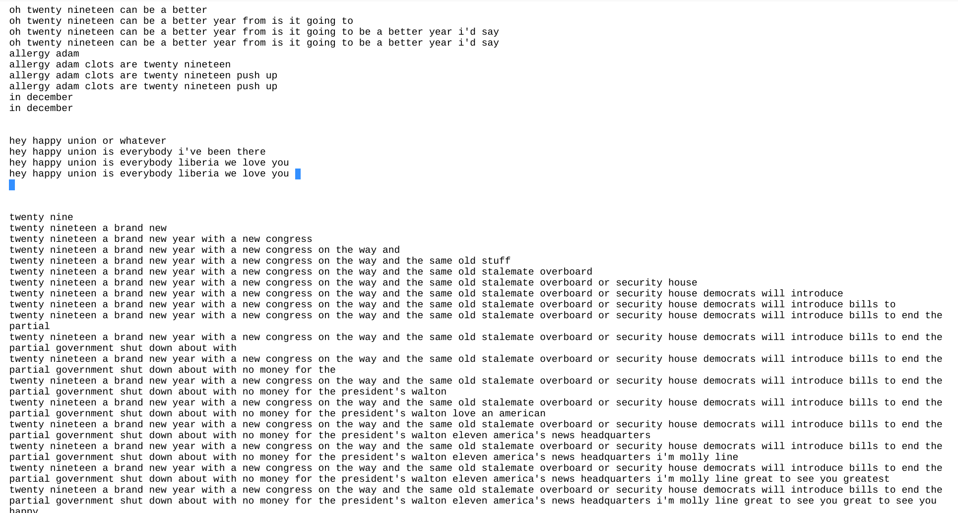
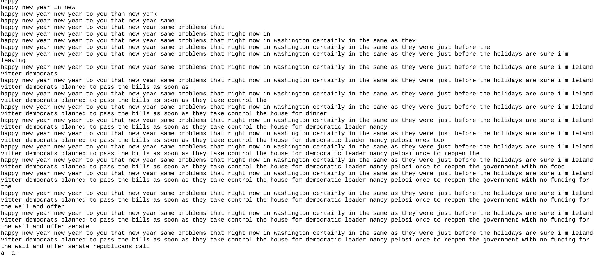
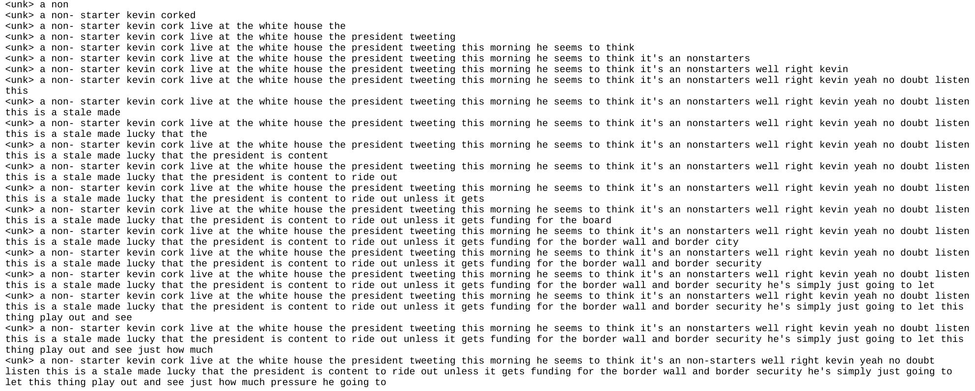
This returns the transcript, for a sample demo, a news file transcript output is shown below , You can click on the image or here to listen to the original audio:

The transcript generated for the same by the engine is provided below in the order of metric of growth :

Future Work

At present, the Indian English is trained along with the NPTEL model, though this provides a substantial level of accuracy. There needs to be more works done to enhance the accuracy on same. Speaker Diarization is one aspect that needs to be perfected to improve the accuracy levels by splitting speaker wise. More data needs to be collected on that domain to make it accurate. Other improvements include, training the same datasets on different neural network architectures to optimize it for a higher Word Error Rate. A semi - supervised learning engine can be trained by leveraging this existing model to enhance the accuracy in the next step.

References

• D. Povey, A. Ghoshal, G. Boulianne, L. Burget, O. Glembek, N. Goel, M. Hannemann, P. Motlicek, Y. Qian, P. Schwarz, J. Silovsky, G. Stemmer, and K. Vesely. ”The Kaldi Speech Recognition Toolkit”. In IEEE 2011 Workshop on Automatic Speech Recognition and Understanding. IEEE Signal Processing Society, 2011.

• V. Peddinti, D. Povey, and S. Khudanpur, “A time delay neural network architecture for efficient modeling of long temporal contexts,” in Proceedings of INTERSPEECH, 2015.

• D. Povey, V. Peddinti, D. Galvez, P. Ghahrmani, V. Manohar, X. Na, Y. Wang, and S. Khudanpur, “Purely sequence-trained neural networks for ASR based on lattice-free MMI”, in Proc. Interspeech, pp. 2751–2755, 2016.

• “A Symmetrization of the Subspace Gaussian Mixture Model”, Daniel Povey, Martin Karafiat, Arnab Ghoshal, Petr Schwarz, ICASSP 2011

• “Revisiting Recurrent Neural Networks for Robust ASR”, Oriol Vinyals, Suman V. Ravuri, Daniel Povey, ICASSP 2012